
Valuation Bible (extended)
Most investors use the P/E ratio like a shortcut: low = cheap, high = expensive.
That shortcut is exactly how you end up buying value traps… and selling compounders too early.
The missing piece is ROIIC. Once you connect growth to reinvestment and returns on incremental capital, you realize a wide range of P/E multiples can be perfectly fair — and the real question becomes capital allocation + time horizon.
The Valuation Bible explains the holy grail behind growth, capital allocation, and valuation.

Part 1 challenges the way most investors use the P/E ratio. Instead of treating the multiple as “cheap” or “expensive” in isolation, we focus on what truly drives long-term returns:
(1) how much of a company’s profits are reinvested, and
(2) the return on incremental invested capital (ROIIC) it can earn on those reinvestments.
The key idea: a wide range of P/E multiples can be “fair” once you understand the reinvestment/ROIIC profile behind them.
Part 2 turns these insights into a simple valuation framework. Using the 3 Engines Model – later extended to 4 Engines with dividends – we decompose total shareholder return (TSR) into:
(1) earnings growth,
(2) changes in share count,
(3) multiple expansion/contraction, and
(4) dividend payments.
Across the scenarios, one pattern is consistent: high ROIIC plus high reinvestment tends to produce superior TSR, while low ROIIC usually argues for cash distributions rather than chasing growth.
In the end, everything comes back to two pillars: capital allocation and time horizon.
🎁 Bonus: If you want to play around with the numbers in our hypothetical example discussed herewith, you can download the Template at the end of the article.
Part 1: The P/E Ratio Misconception — Or: Not All Value Is Created Equal
The Efficient Market Hypothesis states that all available information is fully reflected in current market prices. This means (in theory!) that investors cannot systematically achieve excess returns, because new information is immediately priced in.
However, real-world experience tells a different story. How else could we explain that stock prices often fluctuate by 50 % between their 52-week highs and lows, even for multi-billion-dollar companies? Think of Meta in 2022/2023.
Investors often assume the following:
(1) a low P/E indicates undervaluation
(2) a high P/E indicates overvaluation
However, this approach is flawed because it ignores the role of Return on Incremental Invested Capital (ROIIC).
This divides the investment community into two camps: value investors and growth investors.
Value investors focus on finding undervalued stocks. A better description would be “arbitrageurs”, because classical value investors search for arbitrage opportunities where the market price has significantly deviated from the company’s intrinsic value. This assumes that the market has mispriced the company.
Value investors often concentrate on companies with low P/E ratios, hoping to generate strong performance through multiple arbitrage over a short time frame (i.e. generating their investment return primarily through a change in the valuation multiple rather than underlying earnings growth).
While this approach can work well for some investors, it comes with several weaknesses:
Many value investors crowd this space, increasing competition among investors and making it harder to find opportunities.
These companies are often of lower quality, increasing the risk of value traps.
Shorter investment horizons lead to higher portfolio turnover, requiring more work to monitor a larger number of companies. This process is less repeatable compared to focusing on high-quality businesses and thereby selectively excluding >95% of all companies.
Higher portfolio turnover increases reinvestment risk: the more decisions you have to make, the greater the probability of making mistakes.
Therefore, Slow Compounding exclusively focuses on high-quality companies.
Determinants of Company Value
The common practice for company valuation is based on a Discounted Cash Flow (DCF) model:
A company’s value is the sum of all future cash flows attributable to shareholders (free cash flow), discounted back to their present value.
A simple DCF model is the Gordon Growth Model (Dividend Discount Model).
It is based on the idea that the value of a stock is the present value of all future. dividend payments.
Importantly, we assume here that “dividends” include not only cash dividends but the free cash flow — that is, all profits not reinvested into the business and thus available to shareholders.
The formula shows that the price of a company (P) is determined by three variables:
The dividend in the next year (D1)
The future growth rate of this dividend (g)
The discount rate (r) used to calculate the present value
For example, if we assume that a company will pay a dividend of $1 next year, that the dividend will grow annually by 5%, and that the discount rate is 10%, then the value of the infinite stream of dividends would be:
At a P/E ratio of 20x, the stock would be fairly valued (20 / $1). If you could buy the stock at a lower multiple (for example $16) and wait for the market to recognize the undervaluation, this would be a classic value-arbitrage play (with a 25 % gain after re-rating).
The discount rate we use is the expected return on investment — the cost of equity. This represents opportunity cost: the foregone benefit of the next best alternative.
It is important to note that the Gordon Growth Model has several limitations:
It assumes a constant dividend growth rate (g), even though this fluctuates in reality (and of course is difficult to forecast precisely)
It assumes a stable capital structure, although changes in leverage would influence the cost of equity (r)
The model does not work if g > r, because that would lead to a negative denominator
Interestingly, the variable D1 is often neglected. Investors think a lot about g and r, but pay little attention to D1.
In the simple formula above, the three variables appear independent. In reality, there is a close relationship between D1 and g. Ignoring this connection leads to the incorrect interpretation of the P/E ratio!
Simply put: The more a company must reinvest to achieve a certain growth rate, the less free cash flow remains — and vice versa.
Thus, D1 is not an isolated figure. Whether D1 is high or low depends on how much and at what return a company reinvests part of its profits to achieve earnings growth.
The Importance of ROIIC
Earnings growth can be very simply expressed as:
Whereas:
Reinvestment Rate (herafter: RR) describes the proportion of earnings that is reinvested (e.g., into organic growth or M&A).
ROIIC represents the incremental profit generated for each additional dollar invested.
To make this more concrete, let’s look at two hypothetical companies, A and B.
Both generate earnings per share (EPS) of $1 and both aim to grow earnings by 5% next year.
Both must reinvest part of their profits. How much they need to reinvest depends on the ROIIC they can achieve on those investments.
Suppose Company A achieves an ROIIC of 25%.
To grow profits by 5%, it must reinvest:
In other words, reinvesting 20% of profits at a 25% ROIIC results in 5% earnings growth (20% × 25% = 5%). Thus, Company A has 80 cents left in free cash flow ($1 of earnings minus 20% reinvestment) that can be distributed to shareholders.
Company B, on the other hand, only achieves an ROIIC of 10%. To achieve the same 5% earnings growth, it must reinvest:
Thus, only 50 cents remain as free cash flow for shareholders.
Assuming a cost of capital (r) of 10%, we can calculate the fair values for A and B:
Since both companies have $1 EPS, the fair P/E for Company A is 16x, while for Company B it is 10x.
A traditional value investor might argue:
“Both companies are growing at the same rate. Company B is cheaper than A, so I’m buying B and will wait for a rerating to a P/E of 16 like Company A.”
This reasoning is flawed.
Even though both companies have the same earnings and growth rates, they are not equally valuable according to the Gordon Growth Model. Thus, they should not trade at the same P/E.
Why?
Because they achieve different returns on incremental invested capital.
We can slightly rearrange the Gordon Growth Model. We also know already:
And:
So:
We also know that:
Therefore:
Thus, by substituting these into the Gordon Growth Model, we get:
We can apply the formula for Company A to demonstrate what we have calculated manually already:
Think of the reinvestment rate as the opposite of the distribution (payout) rate.
The higher the reinvestment rate, the lower the free cash flow available for distribution.
The lower the reinvestment rate, the more free cash flow remains for distribution.
At a given expected growth rate, companies with a higher ROIIC tend to distribute a greater portion of their earnings compared to a company with a lower ROIIC.
This impacts D1 in the Gordon Growth Model, leading to higher initial dividends (and thus a higher valuation) because less capital needs to be reinvested to achieve the desired growth.
Let’s summarize what we have learned so far:
High ROIIC → Lower reinvestment rate needed → Higher Free Cash Flow → Higher Value
Low ROIIC → Higher reinvestment rate needed → Lower Free Cash Flow → Lower Value
Interpreting P/E Ratios Correctly
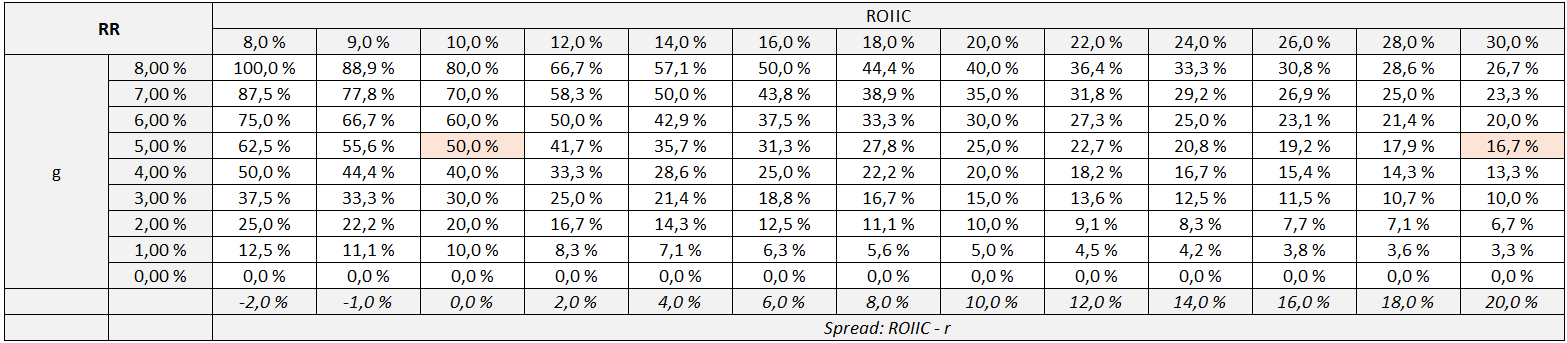
Let’s now look at a set of hypothetical scenarios based on combinations of ROIIC (which affects D1) and g (the growth rate). The outcome is shown in Table 1. Whereas Table 2 shows the reinvestment rate (RR), which can be implicitly derived from Table 1 (RR = g / ROIIC).
Each column also shows the spread between ROIIC and r, which helps in understanding what happens when ROIIC is higher or lower than the cost of capital (as we will discuss in a minute).
In our example, we hold the discount rate (r) constant at 10%. Each scenario assumes EPS = $1, so the resulting price also directly represents the corresponding P/E ratio.
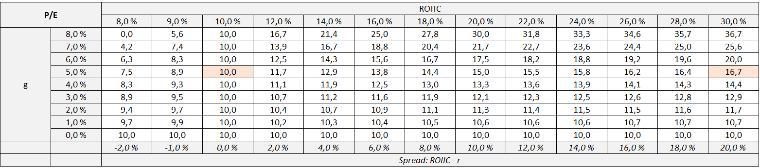
Just cross-check what we calculated for Company B above, growing 5 % with a ROIIC of 10 %. You find the P/E of 10 in Table 1 and the implied Reinvestment Rate of 50 % in Table 2 (you will not find the numbers for Company A, as the table does not show a ROIIC of 25 %. But you could find them if you change the ROIIC to 25 %, of course).
You might be overwhelmed by the number of figures in these tables, but don’t worry…
Let’s analyze Table 1 in more detail in a minute. Before doing so, we need to clarify one more important thing:
One of the most important insights from Table 1 is that the P/E ratio, when viewed in isolation, does not provide a reliable indication of whether a company is cheap or expensive.
Just look at the wide range of results from 0.0x to 36.7x — and remember that, according to the Gordon Growth Model, all of these companies would be fairly (!!!) valued at those multiples!
As we like to say:
Cheap is cheap for a reason, and expensive is expensive for a reason!
As mentioned earlier, D1 and g are connected through ROIIC.
Thus, companies face a dilemma:
To grow faster, the reinvestment rate must increase. This leads to a…
…lower numerator (because D1 decreases due to higher reinvestment), and
…lower denominator (because g increases, so r-g decreases).
If a company accepts slower growth…
…the numerator remains higher (since higher D1 is available for distribution), and
…higher denominator (because g is lower, so r-g increases).
From a mathematical standpoint, a company’s value can increase in two ways:
By increasing the numerator (D1), or
By reducing the denominator (r – g), that is, by increasing the growth rate g.
In other words:
A lower reinvestment rate results in a higher payout ratio, but must be accepted at the cost of a lower growth rate.
Let’s now take a close look at Table 1 and systematically analyze the results to determine which of the two effects (impact on numerator vs. denominator) has the greater influence on company value.
We start with the bottom row; g = 0%.
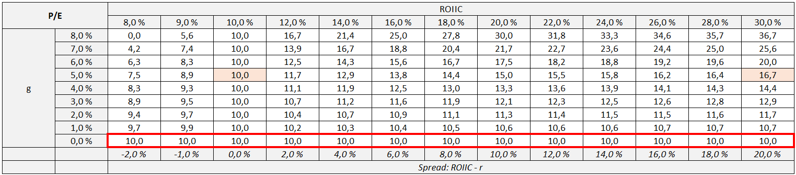
The company does not aim to grow. As a result:
No reinvestment is necessary.
The payout ratio across all scenarios is 100% from left to right because ROIIC plays no role as the reinvestment rate is 0%.
A growth rate of 0% means that all future dividends are equivalent to D1.
The stock is priced like a perpetual bond, fairly priced at $10 as it yields 10% p.a.
Next, let’s consider scenarios with positive growth:
First, we look horizontally across a row (constant growth rate, increasing ROIIC). Let’s choose 5 % for instance:
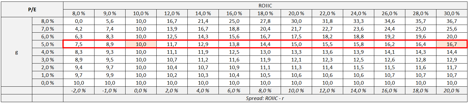
The company’s value and its P/E ratio increase as ROIIC increases, no matter which growth rate we consider.
This is logical: The higher the ROIIC, the less reinvestment is needed to achieve the same growth.
Just because two companies have the same growth rate does not mean they should trade at the same P/E multiple! Any peer comparison that ignores ROIIC is misleading and leads to false conclusions!
Next, let’s look at constant ROIIC.
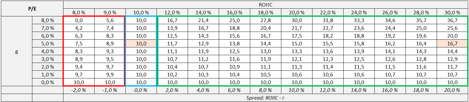
If we move vertically within a column (constant ROIIC, varying growth rates), the outcome depends on whether the ROIIC spread (ROIIC less r) is positive, negative, or zero:
Positive ROIIC spread (green frame above):
Faster growth increases company value and the fair P/E ratio.
As a result, the fair P/E ratio is >10x.
The greater the ROIIC spread, the more sensitive the fair P/E ratio becomes to increases in growth. Example:
With a ROIIC spread of 2%, increasing growth from 3% to 6% raises the fair P/E from 10.7x to 12.5x (+17%).
With a ROIIC spread of 20%, the same growth increase raises the fair P/E from 12.9x to 20.0x (+55%).
Negative ROIIC spread (red frame above):
This seems bizarre but is logical:
If the ROIIC is lower than the cost of capital, faster growth destroys value.
Thus, the fair P/E ratio declines as growth increases.
As a result, the fair P/E ratio is <10x.
Table 1 even illustrates an extreme scenario where a company’s value drops to zero. For instance, if a company grows its earnings by 8% but achieves a ROIIC of only 8%, it must reinvest 100% of its earnings to sustain that growth. As a result, the payout ratio falls to 0%, leaving no free cash flow available for shareholders. Since D1 becomes zero, the company ultimately generates no distributable cash flow at any point. In such a case, the business is practically worthless because it never provides shareholders with positive free cash flow.
Zero ROIIC spread (blue frame above):
If ROIIC equals the cost of capital (r), the company can grow as fast as it likes without impacting its value.
Growth is value-neutral.
As a result, the fair P/E ratio equals 10x, regardless of the growth rate.
Let’s return to the question of which effect has the stronger impact on company value:
The decisive factor is the ROIIC spread:
With a negative ROIIC spread, the decrease in the numerator (D1) is greater than the decrease in the denominator (r-g) driven by a higher growth rate.
Conversely, with a positive ROIIC spread, the decrease in the numerator (D1) is smaller than the decrease in the denominator (r-g) driven by a higher growth rate.
When the ROIIC spread is zero, both effects balance each other out.
To make this even more tangible, let’s revisit the example with a +10% ROIIC spread, where we increase the growth rate from 5% to 8%.
At 5% growth, we arrive at a P/E of 15 (as also shown in the table).
At 8% growth, the implied P/E doubles to 30:
Intuitively, the numerator declines as growth increases (because higher growth implies a higher reinvestment rate). In this example, the numerator falls by 20% (from $0.75 to $0.60). At the same time, the denominator also declines as growth increases — but here it falls by 60% in relative terms (from 5% to 2%).
Whenever the denominator shrinks more than the numerator, the overall value increases — which is exactly what you see here in the jump in the P/E from 15 to 30.
ROIIC vs. ROIC
You may have noticed that we have consistently referred to ROIIC so far, not ROIC.
ROIC generally reflects the return a company achieves on capital that was invested in the past — often many years ago. We could also call it “rolling ROIC”.
ROIIC measures the profitability of newly invested capital over a given period.
Obviously, a company that produces a high ROIC is a good business. However, it only tells us the rate of return the company is generating TODAY on capital that has already been invested in the PAST (sometimes many years ago).
But what is far more important is how much return the company can generate in the future with new capital investments.
A high historical ROIC indicates past success. However, the stock market prices the future, not the past. Thus, future ROIIC is what truly matters for shareholder value creation.
If Company X achieved a historical ROIC of 15% but no longer has attractive reinvestment opportunities at a comparable ROIIC, while Company Y also has a ROIC of 15% and still enjoys many reinvestment opportunities at 15% ROIIC, then Company Y deserves a valuation premium over Company X, despite both generating a 15 % ROIC.
A high ROIC is an indication of an existing economic moat.
However, what ultimately counts is the future. What matters is the ROIIC a company can achieve in the future.
ROIC tends to be a backward-looking measure (past performance), while ROIIC provides a forward-looking perspective (future returns). Nevertheless, ROIIC can also be calculated for a specific historical period.
Let’s consider a simplified example:
Suppose a company has invested capital of $100 million at the beginning of the observation period and $300 million at the end. Over the same period, it cumulatively generated $400 million in earnings, while the company’s annual earnings increased by $50 million between the beginning and end of the period under review.
Put simply, retained earnings increase invested capital, while dividend payments or share buybacks reduce invested capital. Hence, we can calculate both ROIIC and RR:
ROIIC:
Invested capital increased by $200 million, while earnings increased by $50 million. Hence, ROIIC would be 25 %.
RR:
Invested capital increased by $200 million, while cumulative earnings totaled $400 million, resulting in a reinvestment rate of 50%.
This would result in an average earnings growth rate of approximately 12.5% per year (25% ROIIC × 50% reinvestment rate).
Walmart’s ROIIC
Let’s now apply this to a real-world example.
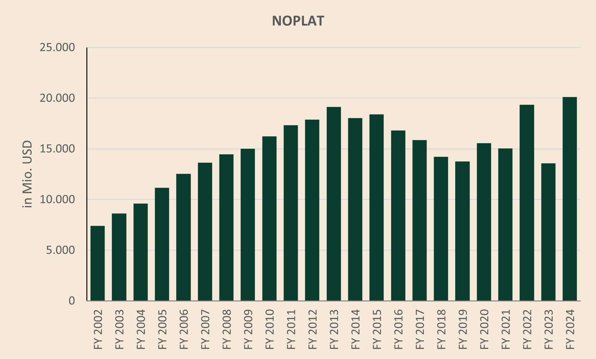
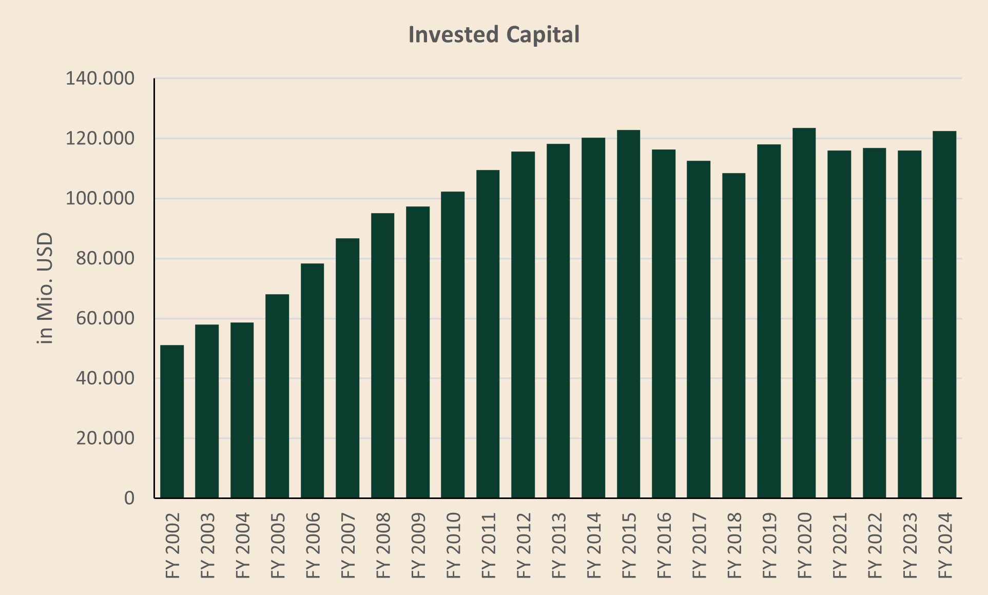
Walmart achieved a NOPLAT (Net Operating Profit Less Adjusted Taxes) of $7.4 billion in fiscal year 2002, while invested capital (equity plus financial debt excluding lease liabilities minus cash) stood at around $51.0 billion.
This translates into a ROIC of 14.5% — not bad, as Walmart earned well above its cost of capital.
By fiscal year 2024, Walmart’s NOPLAT had grown to $20.1 billion, while invested capital increased to $122.4 billion.
Over the entire observation period, Walmart generated cumulative NOPLAT of $323.5 billion.
and
Over the full period, Walmart thus:
Reinvested approximately 22% of its earnings at a ROIIC of about 18%.
This resulted in an earnings growth rate of approximately 4.0% per year (17.8 % x 22.1 %), which closely aligns with the NOPAT compound annual growth rate (CAGR) of 4.7%.
It’s important to note that the selection of the period under review (FY2002-FY2024) was purely coincidental.
A more interesting question is whether Walmart’s reinvestment rate (RR) and ROIIC changed over time.
The two charts below show the development of NOPLAT and Invested Capital.
Both charts indicate that a peak was reached between 2013 and 2015, after which the figures eroded, with NOPLAT becoming particularly erratic.
We can confirm this development through the lens of ROIIC and RR as well.
Instead of only looking at the longest observation period from FY2002-FY2024 (as we did previously), the following matrix shows the reinvestment rate for all possible combinations of starting and ending years.
We perform this calculation to make changes in reinvestment rates over time visible.
Horizontally, the matrix shows the starting year of the observation period.
Vertically, it shows the ending year.
The black diagonal lines represent 5-year periods.
In the top left corner, we find the result we already calculated earlier for the period FY2002–2024.
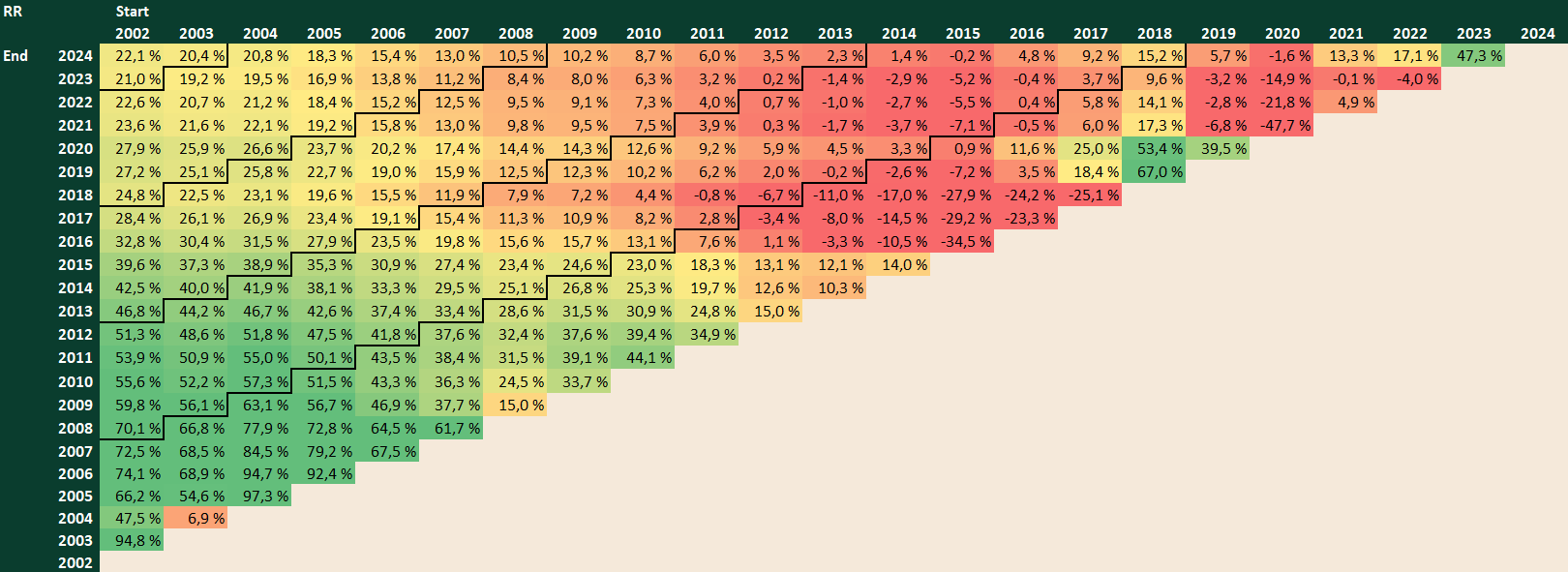
In general, we can say: the longer the observation period, the more accurate (and meaningful) the calculation, which is also reflected in the color shading.
The shorter the observation period, the more erratic the results, and the lower their significance.
This is because, over short periods, there are naturally other influences on earnings growth that cannot be directly attributed to the reinvestment rate (RR) or ROIIC.
If we look at the first column with the start year 2002, we observe that the reinvestment rate decreases as we move upward (i.e., as the observation period shortens).
Thus, the longer the observation period in Walmart’s case, the higher the reinvestment rate becomes.
This implies that Walmart’s reinvestment rate has declined over time.
To verify this and to align it with the stagnating developments in NOPLAT and invested capital, we examine two consecutive periods:
FY2002-Y2014 (peak year): The reinvestment rate was 42.5%.
FY2014-Y2024: The reinvestment rate dropped to only 1.4%.
That’s why we initially calculated a 22 % reinvestment rate for FY2002-FY2024 (which reflects the average of 42.5 % and 1.4 %).
I believe that the “Reinvestment Rate triangle” allows a more nuanced analysis of historical RR (also ROIIC).
Conclusion for Part 1
The P/E ratio alone is not a reliable indicator for valuing a company if ROIIC and reinvestment rates are not considered.
A seemingly high P/E can actually offer better value than a low P/E.
Quality comes at a price.
A P/E that is significantly above or below its historical average does not necessarily indicate overvaluation or undervaluation, as Mr. Market may (!) price in a permanent change in RR and/or ROIIC.
ROIIC and RR don’t have to be constant and may change over time (in either direction).
Therefore, it is crucial to examine how ROIIC and RR have evolved over time (which cannot be immediately inferred from simply looking at ROIC).
Part 2: Valuation Framework — Or: Distilling Shareholder Returns
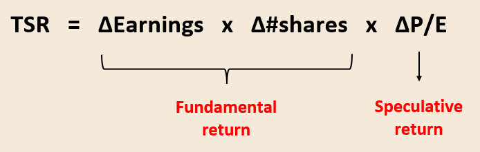
Fundamental vs. Speculative return
Simply put, total shareholder return (TSR) consists of two components:
Fundamental return
Speculative return
The fundamental return is based on the operational earnings development of the underlying company and its distribution policy (dividends / share buybacks).
The speculative return, on the other hand, is based on changes in the multiple that Mr. Market assigns to the company’s earnings and cash flow streams.
We already outlined in Part 1 that the level of the fair multiple should depend on the company’s reinvestment opportunities and its ROIIC, in theory.
However, in practice, the actual multiple is influenced by various factors and fluctuates, rather than remaining constant.
While today’s earnings level and distribution policy are known variables, the multiple reflects several unknown and subjective variables, making it much more dependent on investor perception.
Investor perception has no “limit” as to how much it can fluctuate over any given time period.
For this reason, over short investment horizons, it is the multiple that determines shareholder returns. Over longer periods, however, earnings growth becomes the most important factor.
Buybacks and dividends aside, the share price should reflect the growth in earnings. A change in the multiple acts like a headwind or a tailwind.
Multiples tend to fluctuate within a certain range,
Earnings can grow steadily over years and exhibit “unlimited” upside potential.
Over longer periods, earnings growth can far outpace multiple expansion.
When we speak of multiple expansion or multiple contraction, we refer to the change of valuation multiples between two points in time. A multiple expansion has a positive effect on TSR (tailwind), while a multiple contraction negatively impacts TSR (headwind).
The change in multiples is unpredictable and depends on many factors. However, the further into the future we look, the less relevant changes in multiples become, as earnings growth outweighs the impact of minor changes in multiples.
Example: Lagercrantz Group AB
Let’s take a look at Lagercrantz Group AB, a Swedish serial acquirer (which I will cover in more detail in an upcoming deep dive), to demonstrate the fundamental concept behind long-term shareholder value creation.

Over the last 10 years, the stock is up ~8x (~700 %), or ~23% p.a, while Net income is up ~5.8x (~480 %), or ~17% p.a. Over the same period, the P/E increased from 19.6x to 35.1x currently, which translates into a tailwind of +6% p.a, closing the gap. To summarize it:
Earnings growth: +17 % p.a.
Multiple inflation: +6% p.a.

Over long periods, I would argue that for quality companies…
…earnings growth is more predictable than changes in multiples, and
…earnings growth is something that management can at least partially control.
What drives investment results?
Let’s have a look at what drives investment results:
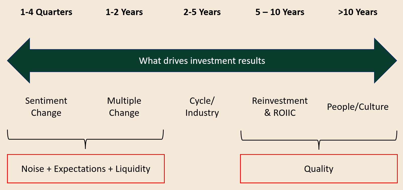
In the short term, the following factors (among others) drive stock prices:
“Noise” & Changing perceptions among investors: For instance, Earnings beats/misses vs. consensus, daily macro headlines, inflation and unemployment reports, geopolitical headlines with no real earnings impact, whether the FED is keeping interest rates stable (just to name a few).
Liquidity issues: For instance, weak performance of European small-caps due to many asset managers facing outflows and indiscriminately selling off assets.
Over the long term, the key determinants for investment results are the reinvestment strategy and corporate culture.
The multiple is also heavily influenced by the predictability and reliability of the underlying profit streams.
The more predictable and reliable an earnings stream, the less risky and the higher the valuation multiple that Mr. Market can assign to the stock.
A theoretical (and perhaps utopian) example would be a company that we know can increase its profits by 10% annually for the next 100 years for sure. We could then calculate the multiple that we could assign to such a company in order to achieve an 8% return.
Let’s assume the company starts with a profit of $100. With a 10% annual growth over 100 years, the final profit would be $1.38 million. The present value (PV) of this company’s cash flows (without considering terminal value), discounted at the required IRR of 8%, would be $29,044. This means we should be willing to pay 290 times the current profit (PV of future cash flows/current profit) if we aim for a CAGR of 8% over the next century. In other words, we could pay an extremely high multiple and still make money.
However, there’s a catch: The real world doesn’t align with our utopian scenario.
The real world changes permanently. Companies come and go (bust). Industries are disrupted by new technology (“I believe in the horse, the automobile is a temporary phenomenon”, as Emperor Wilhelm II said before cars stole the market shares from horse-drawn carriages).
The future is uncertain. Returns 20 years from now aren’t guaranteed, let alone 100 years down the line. This implies that investors should have a realistic understanding of how returns might evolve in the future, always erring on the side of caution (and not on the optimistic side).
One way to achieve this is by breaking down the drivers of profit growth (such as ROIIC and reinvestment rate) in order to better understand what we can reasonably expect going forward.
Let’s zoom out for a moment. We know:
We can further break down the profit as:
Thus, we have:
This means that any change in market capitalization must come from a change (Δ) in one of the individual components:
However, it’s important to note that a change in market capitalization does not translate into a positive Total Shareholder Return (TSR) for the individual shareholder.
To illustrate this, just think of a hypothetical company:
Shares outstanding: 100
Earnings: $200
EPS: $2 ($200 / 100)
P/E: 10
Market Capitalization: $2,000 ($200 x 10)
Stock price: 20 ($2,000 / 100)
Now we assume the company issues new shares and doubles the share count and parks the cash (i.e. no change in earnings). It looks as follows now:
Shares outstanding: 200
Earnings: $200
EPS: $1 ($200 / 200)
P/E: 10
Market Capitalization: $2,000 ($200 x 10)
Stock price: 10 ($2,000 / $200)
As we assume no change in the P/E ratio, the Market Capitalization does not change, as the decrease in EPS and the increase in shares outstanding offset each other (as the underlying earnings do not change). Let’s use the above formula to confirm that the Market Capitalization is unaffected:
TSR is -50 % as the stock price halves!
What matters more for an investor than just the change in the Market Cap is the TSR based on the price per share.
That’s why we cannot use the above formula to calculate TSR. We have to make two adjustments:
For Δ#Shares we use the reciprocal value, i.e. if the share count doubles, we use 0.5x as a multiplier. On the opposite, if the share count halves after buybacks, we use 2.0x as a multiplier.
We have to look at the Earnings instead of EPS, as otherwise we would make a double count.
Don’t get confused here. We will make some examples in a minute.
To summarize it, we use the following formula to break down TSR into its individual components.
We call this the 3 Engines Model.
Referring to the above example:
The formula now correctly takes into account that the investor would have achieved a TSR of -50%.
Additionally, as we discussed in Part 1, we know that the change in earnings is approximately the product of ROIIC and the reinvestment rate.
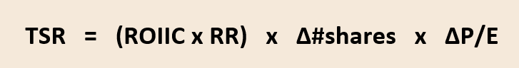
This simple valuation framework helps break down historical TSR into its core components and also provides a way to estimate future returns. For example, a company that reinvests 100% of its profits at a 30% ROIIC, but dilutes shareholders by 50% and sees its multiple cut in half, would have an expected return of roughly 7.5 % p.a.
However, the 3 Engines Model ignores the impact of dividends. After a dividend is paid, shares trade ex-dividend, meaning the share price — and thus market capitalization — drops by the dividend paid out. Essentially, this is just a wealth transfer from the company to the shareholder, unless the dividend drop is offset by price appreciation (ignoring taxes here). When we include dividends in the analysis, we move to the 4 Engines Model.
We’ll now illustrate the entire framework with several hypothetical examples. We’ll look at a five-year period and make different assumptions about reinvestment rates, ROIIC, and capital allocation strategies (dividends, share buybacks, or full reinvestment). We will also set the P/E ratio at t=0 and t=5. For simplicity, we will calculate EPS using the number of shares outstanding at the beginning of the period (meaning any share buybacks occur at the end of the period, based on the starting share price).
Example 1: No Growth; Only Dividends
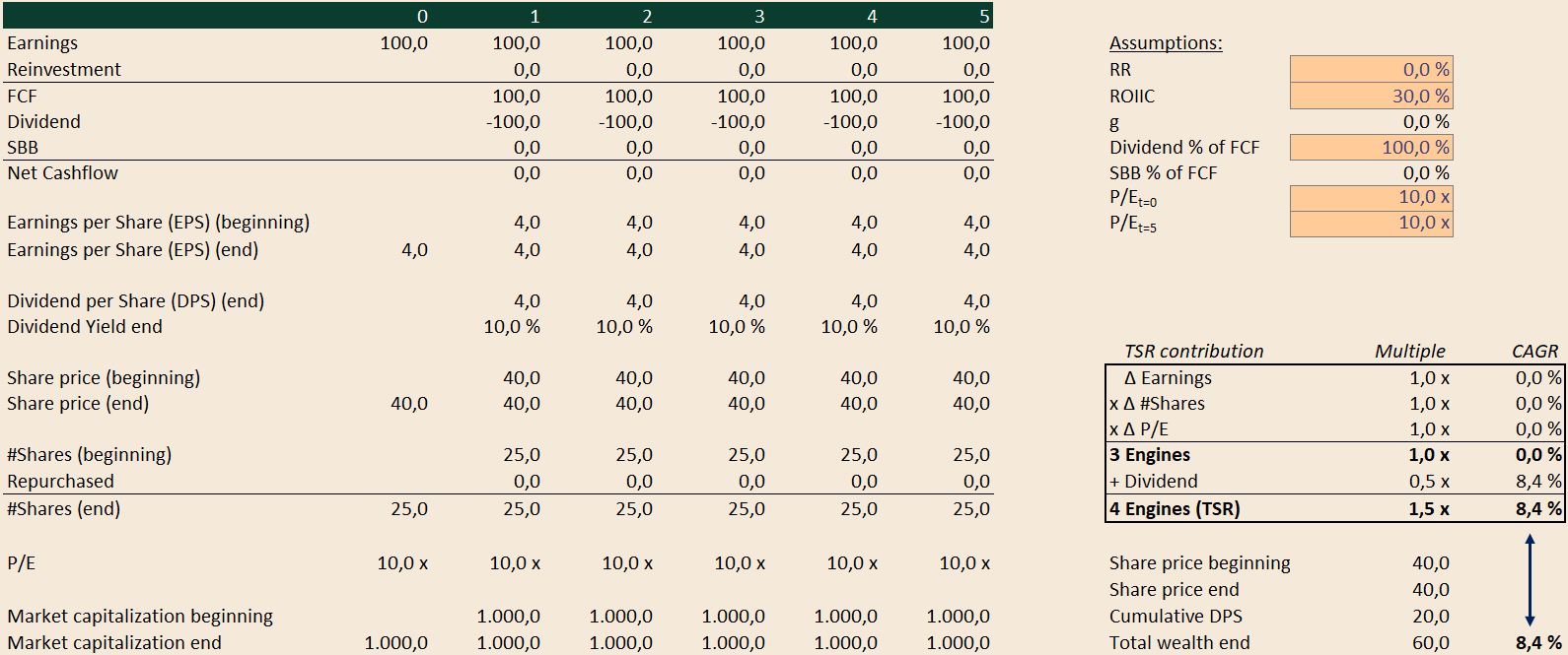
Since the reinvestment rate is 0%, profits remain constant across all periods. No reinvestment is needed, meaning earnings equal free cash flow (FCF). We assume a 100% payout ratio. As we are assuming a constant multiple, each dividend payment is offset by a corresponding increase in the share price (otherwise, mathematically, the P/E ratio would continuously decline).
In this case, the ‘Earnings Engine’, the ‘#Shares Engine’, and the ‘P/E Engine’ each contribute 0% return (as reflected by an unchanged market capitalization and a multiplier of “1.0x”). Over five years, a total of $500 in dividends is paid out, which corresponds to 0.5 times the initial market capitalization at end of year 0. CAGR’ed over five years, this results in an annualized return of 8.4%.
Note that the dividend yield equals 10 %, while the TSR comes in at an 8.4 % CAGR only. That’s because the dividend is not reinvested and thus does not produce any returns.
Example 2: No Growth; Only Share-Buy-Back (SBB)

Similar to Example 1, but with the difference that instead of paying out dividends, the company uses the cash for share buybacks. As mentioned earlier, we calculate the number of shares repurchased based on the share price at the beginning of the period for a simplified calculation.
At t=1, this means $100 of FCF divided by a $40 share price results in 2.5 shares repurchased, reducing the number of outstanding shares to 22.5 by the end of the period (a reduction of 10%, as the shares trade at a P/E of 10).
After the buyback, EPS increases to $4.44, which — assuming a P/E ratio of 10x — leads to a share price of $44.4 at the end of t=1. And so on and so forth for the remaining years.
Again, we observe that market capitalization remains unchanged because we assumed that share repurchases affect the share count at the end of the period, which boosts EPS and, accordingly, lifts the share price.
Another very interesting observation is that despite the same amount of FCF being distributed over 5 years ($500), the TSR is higher than in the Dividend Scenario and exceeds the FCF-Yield of 10 %. That’s because the ownership in the company increases by 11.1 % per year. Imagine you own 1 of the 25 shares (4 % ownership) in our example. After buying back 10 % = 2.5 shares, the share count decreases to 22.5. You still own 1 share, hence your ownership increases to 4.44 %. That’s a 11.1 % increase.
When we increase the P/E ratio from 10x to 20x across all years, we can observe that the TSR drops significantly (see example 2b below).

This makes perfect sense: with all other assumptions held constant, a higher valuation means the company can repurchase fewer shares with the same amount of FCF, reducing the impact of buybacks on EPS growth and, consequently, on TSR.
Example 3: 100 % Reinvestment Rate; 30 % ROIIC
Now, we assume that 100% of the earnings are reinvested. As a result, the free cash flow (FCF) is zero in all periods. The TSR in this case is 30% per year, fully driven by profit growth.
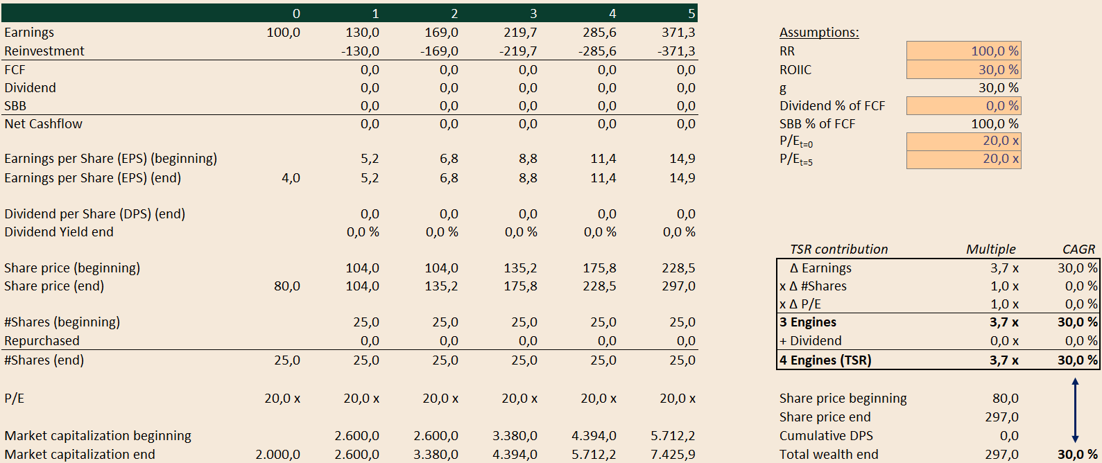
This scenario delivers the highest TSR among the examples we’ve calculated so far.
However, despite the strong TSR, the stock appears expensive when measured against FCF after growth capex, as the FCF yield is 0%!
Traditional value investors might typically avoid such a stock, since it looks unattractive from an FCF-yield perspective.
We can summarize our observations in the following scenario matrix, analyzing different combinations of reinvestment rates and P/E ratios. We are calculating the matrix under the dividend scenario — meaning that any earnings not reinvested are fully distributed as dividends. Additionally, we assume no change in the multiple over time.
In the matrix below, we can already recognize the 10.7% return we calculated in Example 1 (0% reinvestment rate and a P/E of 10) and 30.0 % of Example 3 (100 % reinvestment rate and a P/E of 10).
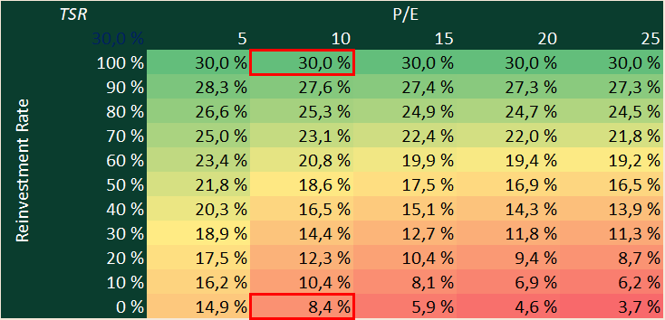
The matrix clearly shows:
If a company can achieve a high ROIIC (30% in this case), the best course of action is to reinvest 100% of its earnings. Without any change in the multiple, the TSR will then equal its earnings growth rate (100% reinvestment rate × 30% ROIIC). There is no scenario that would generate a higher TSR (unless reinvestment rate is increased >100 % through debt financing for instance).
As the reinvestment rate gradually decreases, the TSR becomes increasingly dependent on the P/E ratio. This makes perfect sense: a lower P/E means a lower valuation and thus a higher dividend yield, which helps offset the lower growth.
If we run the same calculation again, but assume a ROIIC of just 5% instead of 30% (meaning the company does not earn its cost of capital), the picture changes dramatically:
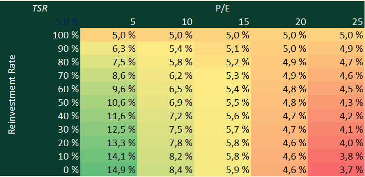
In this case, it’s clearly better for management not to reinvest at all and instead distribute all profits to shareholders.
This directly confirms what we already derived in Part 1 from a different angle:
When the ROIIC is too low, it is better not to reinvest, but rather return earnings to shareholders.
🎁 Bonus: If you want to play around with the numbers, you can download the Template here:

Conclusion for Part 2
Changes in a company’s market capitalization can be broken down into three drivers: Earnings per Share (EPS) × Number of Shares × P/E Multiple.
However, changes in market cap do not automatically translate into changes in shareholder wealth (TSR).
To properly reflect the shareholder perspective, we must adjust for share count changes using the reciprocal of Δ#Shares.The 3 Engines Model was introduced to separate TSR into:
Earnings Growth (linked to ROIIC × Reinvestment Rate).
Share Count Changes (buybacks or dilution).
P/E Multiple Changes.
Dividends transfer value from the company to shareholders without changing underlying market cap growth. Factoring them in leads to the 4 Engines Model.
Examples:
Pure dividends (no growth, no buybacks) yield a steady return based purely on the dividend yield.
Buybacks can improve TSR by reducing share count, but are less effective at higher valuations.
Full reinvestment at high ROIIC produces the highest TSR
Full reinvestment at low ROIIC destroys value, and distributing earnings becomes the better strategy.
Key Insights:
If ROIIC is high, reinvest everything.
If ROIIC is low, distribute cash.
Lower P/E means higher TSR potential through dividends.
In the end, investment results will boil down to a) investment horizon and b) the underlying performance of the business, driven by capital allocation. The shorter your investment horizon, the less attractive quality stocks will be, and the higher the perceived risk of multiple contraction.