
You Have Probably Never Looked at a DCF Like This Before
Why standard DCFs can be too conservative for durable high-growth compounders

This article started with my current research for an upcoming Deep Dive (btw, it’s a wonderful business, so stay tuned).
While working through the company, I kept coming back to the same questions lately: how long is the real growth runway? When does above-average growth fade? And what does that mean for valuation if a standard DCF forces the business into a low terminal-growth assumption too early?
What began as a quick note on terminal value and growth duration became a much longer than planned article. But I also think it became much better. The more I worked through the math, the clearer the point became: for durable compounders, the key valuation question is often not the terminal growth rate itself. It is how long the business can avoid becoming a terminal-growth business in the first place.
You can download the Excel file behind the calculations right here:
One quick note before we start: if you are already very familiar with DCF mechanics, you can skip chapters 2 and 3. These chapters are mostly a refresher on present values (PV) and why the terminal value (TV) is simply a shortcut for cash flows beyond the explicit forecast period.
1. How Most Investors Use a DCF
Investors learn to apply a DCF as a valuation model: Forecast the cash flows. Discount them back. Add the TV. Compare the result to the market cap.
PV < market cap? Overvalued ➜ Sell
PV = market cap? Fairly valued ➜ Do nothing.
PV > market cap? Undervalued (with the difference representing the margin of safety) ➜ Buy
Done.
That is technically correct. But, it also hides the million-dollar question behind every DCF: how durable is the growth? How long can the business continue to compound at above-average rates before it truly fades into maturity?
Durability, i.e. time, is one of the key ingredients in the compounding equation. A standard DCF often gives such businesses ten years of explicit growth and then forces them into a low terminal-growth assumption of 2-4%. That can be reasonable for the average mature business. However, it can be far too conservative for a company that still has a long reinvestment runway (exceeding the explicit 10 year growth), pricing power, high incremental returns, and a culture that can keep extending the opportunity set.
The problem is not the DCF math. The math is fine. The problem is that the spreadsheet often ends before the business does.
In this post, I want to look at a DCF in a way that is rarely shown in practice. We will look at the terminal value, the roll-forward mechanics, the return decomposition, the fair value at different points in time, and finally the effect of extending the high-growth period.
We look at an intentionally simple example. Starting free cash flow (FCF) is 100. We use a 8% discount rate and we assume 10% growth. The terminal growth rate is 2%.
1. What is a DCF?
In its simplest form, a company is worth the sum of all future FCFs, discounted back to today. This is necessary because investors are trying to determine what those future cash flows are worth now. Cash received next year is less valuable than cash received today, because today’s cash can be reinvested immediately and future cash flows are less certain. If cash arrives in year ten, it is discounted for ten years. The further away the cash flow, the less it is worth today. The discount rate is the bridge between the future and the present.
However, no one can forecast cash flows year by year into perpetuity accurately. Apple’s growth in 2065? I have no idea. The usual workaround is to model a detailed forecast period first — usually ten years — and then use a simplified and conservative terminal value for everything that comes after. The TV is simply a shortcut for all the cash flows beyond the explicit forecast period.
This means the enterprise value in a DCF consists of two building blocks:
the PV of the FCFs during the detailed forecast period
the PV of the TV.
For the math-gurus among my readers, the DCF can be written like this, where
(FCFt) represents the free cash flow in year (t),
(r) is the discount rate, i.e. the return required by the investor,
(N) is the length of the explicit forecast period, and,
(TVN) is the terminal value at the end of year (N):
The explicit period is the part most investors spend time on. Revenue growth, margins, capital intensity, reinvestment, working capital, taxes. The TV is often treated as a plug at the end. But it should not be viewed as a black box. It is simply a shortcut for all cash flows after the explicit forecast period. So, before getting into the details, let’s recap the math behind the TV:
2. The Terminal Value: A Shortcut for Infinity
We assume that a company generates 100 of FCF today. For the next ten years, FCF grows at 10% per year. After year 10, the company does not stop growing. It simply matures. From year 11 onward, FCF grows at only 2% per year forever.
The chart below shows the first 30 years. For simplicity, only the first 30 years are displayed, but the underlying assumption is that the cash flows continue beyond year 30 into perpetuity.
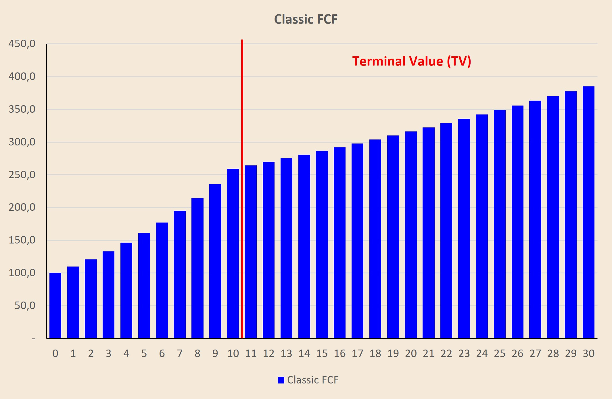
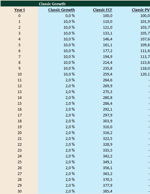
The table then shows the same mechanics in numbers.
Instead of discounting every single cash flow from year 11 to infinity manually, investors use a shortcut: the TV.
In our example, year-10 FCF is 259.4. The first cash flow after the explicit forecast period is therefore year-11 FCF:
The TV at the end of year 10 is then calculated as:
With an 8% discount rate and 2% terminal growth, this gives us:
This 4,409.4 is the value in year 10 of all future cash flows from year 11 onward. It is not yet today’s value. To get the PV of the TV, we still have to discount it back ten years:
This is the shortcut. Instead of forecasting year 11, year 12, year 13, and every year after that into perpetuity, we calculate one TV in year 10 and then discount that TV back to today.
The chart below proves the same point in a more intuitive way. I manually extended the cash flows for more than 250 years and discounted each of them back to today. The cumulative PV of all those post-year-10 cash flows converges toward the same value as the PV of the TV: roughly 2,042.
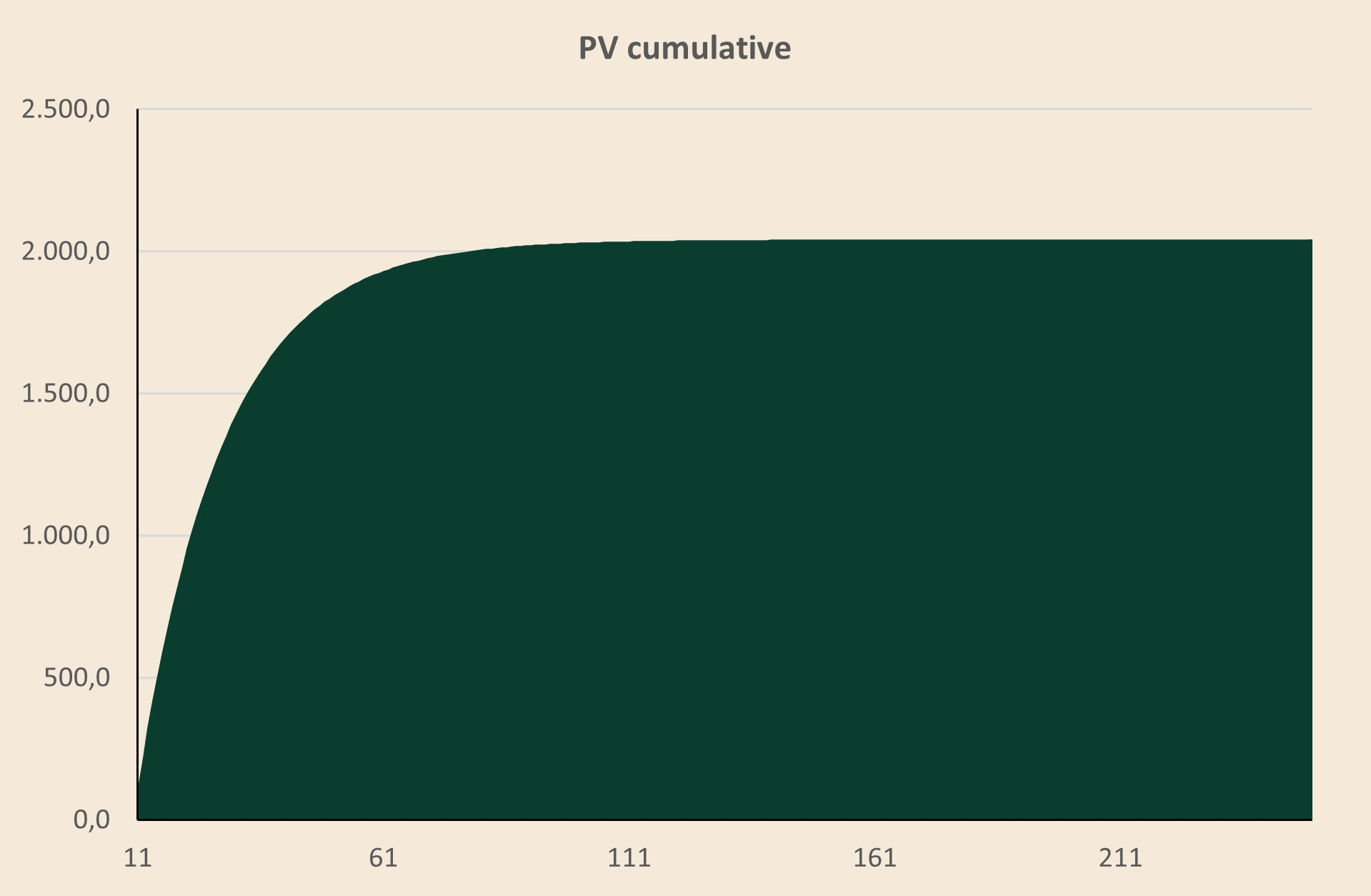
It clarifies what the TV really says, i.e. the classic model does not say the company stops growing after year ten. It says that every cash flow after year ten grows at only 2% indefinetly. That assumption may be perfectly reasonable for many businesses. But, it is also exactly where a DCF can become too conservative for durable high-growth companies.
3. The Base Case: A Fixed 10-Year DCF
With the basic mechanics of a DCF fresh in mind, we can now build the first case step by step.
The value today is the sum of two parts:
In this example, the PV of the explicitly forecast cash flows from year 1 to year 10 is 1,107.7. The TV at the end of year 10 is 4,409.4. Discounted back to today, that TV is worth 2,042.4 (as calculated above).
So the fair value at year 0 is:
That is the base case: a fixed 10-year DCF with ten years of high growth and a 2% terminal growth rate thereafter.
4. The part nobody shows: the DCF roll-forward
Most DCFs stop here. The analyst calculates one fair value today, compares it to the market cap, and moves on.
But that misses a useful second step.
The year-0 fair value of 3,150.1 is only a snapshot. If the business develops as modeled, the DCF starts to roll forward with every year that passes. It evolves over time. Each year, one cash flow is received, the remaining cash flows move one year closer, and the TV is discounted over one fewer year. DCFs are not static!
That is what the roll-forward shows.
The table below takes the exact same fixed 10-year DCF and rolls it forward year by year.
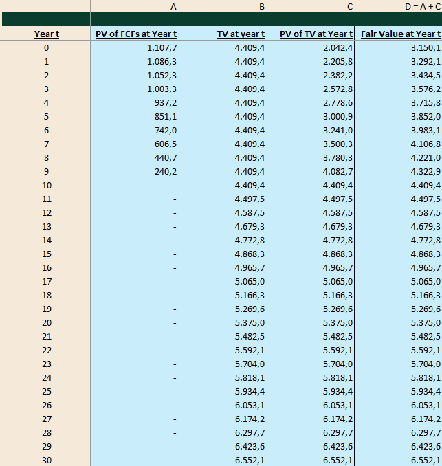
The table breaks the fair value at each point in time into the same two building blocks we used in the year-0 DCF.
Column A shows the PV of the remaining explicit FCFs. At year 0, this is the PV of the cash flows from year 1 to year 10, which equals 1,107.7 (as discussed above). One year later, the year-1 cash flow has already been received, so column A only includes the remaining cash flows from year 2 to year 10. By year 10, the explicit forecast period is fully consumed. There are no high-growth cash flows left to discount separately, so column A falls to zero.
Column B shows the TV. In the fixed 10-year case, the TV is calculated at the end of year 10 and equals 4,409.4 (as discussed above). This number represents all cash flows from year 11 onward, assuming the business grows at 2% forever after year 10.
Column C shows the PV of the TV at each year. At year 0, the terminal value of 4,409.4 is discounted back ten years, so it is worth only 2,042.4 today (confirming what we calculated above). At year 1, it is discounted back nine years. At year 2, eight years, and so on. The closer we get to year 10, the higher the PV of the TV becomes. By year 10, no discounting is left. The PV of the TV equals the TV itself: 4,409.4.
By year 10, the model has used up the entire high-growth period. The fair value then consists entirely of the TV, because from that point onward the company is assumed to be a mature 2% grower.
The chart below visualizes the same mechanics.
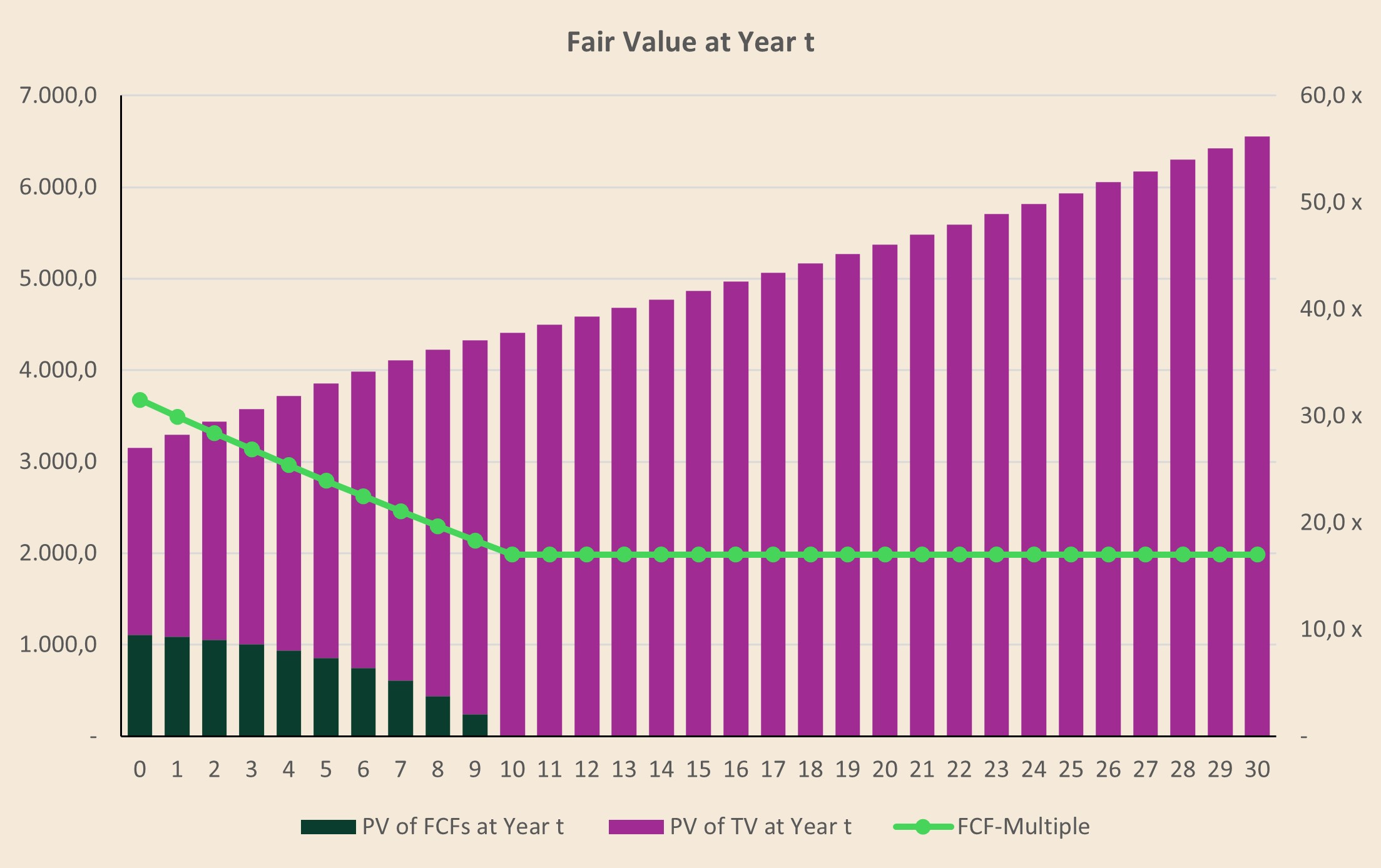
The green bars show the PV of the remaining explicit FCFs (Column A). At year 0, they still contribute 1,107.7 to fair value. As time passes, this component declines because the high-growth cash flows are gradually received and disappear from the remaining DCF. By year 10, the explicit forecast period is fully consumed, so this block falls to zero.
The purple bars show the PV of the TV (Column C). This component moves in the opposite direction. At year 0, the TVis still ten years away and therefore heavily discounted. As we move closer to year 10, the discounting effect becomes smaller. By year 10, the PV of the terminal value equals the TV itself: 4,409.4.
Together, the two bars form the fair value at each point in time (Column D). The composition changes dramatically, but the logic stays the same: fair value is always the sum of the remaining explicit cash flows and the PV of the TV.
Additionally, the green line shows the implied FCF multiple (i.e. the fair value at each year divided by the FCF of that year), assuming the stock trades exactly at fair value at every point in time. It starts above 30x and then declines during the high-growth period. This makes intuitive sense. At year 0, the company still has ten years of 10% growth ahead. By year 5, only five years of high growth are left. By year 10, none are left. The business has mathematically become a mature 2% grower.
From that point onward, the multiple stabilizes. Once the company is in the terminal-growth phase, the valuation is simply a growing perpetuity. With an 8% discount rate and 2% perpetual growth, the value is approximately 17x FCF.
Once the company has entered the terminal-growth phase, the implied FCF multiple is no longer driven by the remaining high-growth runway. It is mechanically determined by the discount rate and the perpetual growth rate.
The terminal value formula is:
Since next year’s FCF equals current FCF grown by (g),
we can rewrite the formula as:
Dividing both sides by current FCF gives the implied current-year FCF multiple:
With an 8% discount rate and 2% perpetual growth, this becomes:
This is why the green line stabilizes at roughly 17x once the company has fully entered the terminal-growth phase.
5. The Return Composition
The previous chapter showed how the fair value evolves over time. Now we can take the next step and look at the return composition.
If the business develops as modeled and the stock trades at fair value at every point in time, the investor’s expected return equals the discount rate. In our example, that discount rate is 8%.
The 8% return has two components:
The table below shows this decomposition year by year.
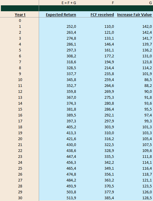
Column E shows the expected return in absolute dollars. This is simply the beginning fair value multiplied by the discount rate.
\(Expected\ Return_t = Fair\ Value_{t-1} \times r\)Column F shows the actual, undiscounted FCF received during the year.
Column G shows the increase in fair value. This is the change in the remaining fair value of the business after the cash flow has been received.
Sounds confusing?
Let’s look at the first year.
At year 0, the fair value is 3,150.1. This is the PV of all future cash flows in the model. Since the model uses an 8% discount rate, the value should roll forward by 8% over the next year as long as the cash flows materialize as assumed.
In other words, one year later, the total value available to the investor should be:
This 252.0 is the return implied by the DCF for the first year. Again, it is the mechanical roll-forward of the PV by one year at the discount rate.
During year 1, the company generates 110.0 of FCF. Once this cash flow has been received, it has to be removed from the remaining fair value calculation, as it is no longer a future cash flow; it is now in the past. The fair value at year 1 therefore only reflects the cash flows that still lie ahead.
At the same time, the fair value of the remaining business increases from 3,150.1 to 3,292.1.
So the total expected return in year 1 is:
Relative to the year-0 fair value, this equals 8% (as expected):
The bridge below shows the same arithmetic visually.
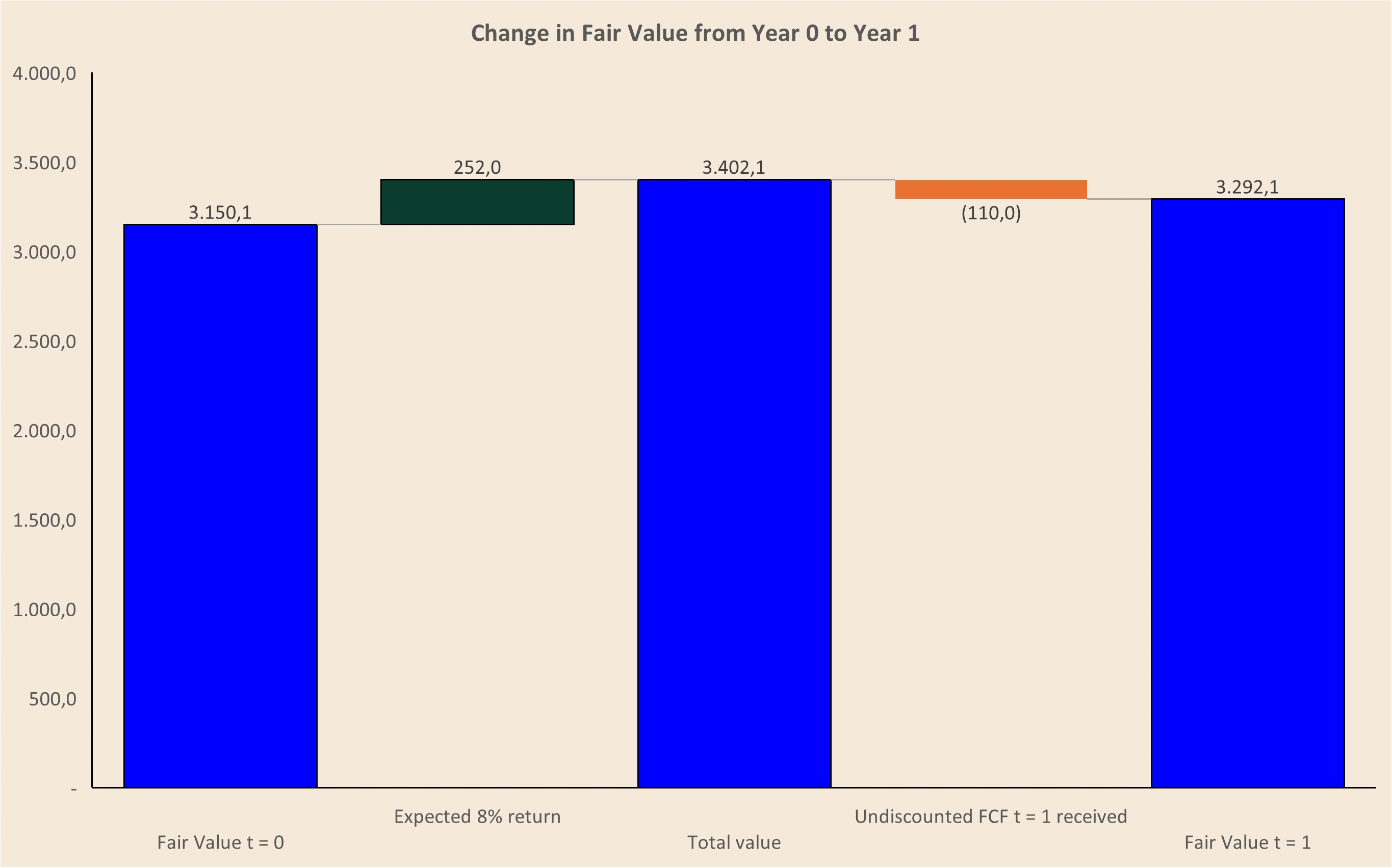
The year-0 fair value of 3,150.1 first rolls forward by the expected 8% return. In dollar terms, that adds 252.0 and brings total value to 3,402.1.
But during year 1, the company also generated 110.0 of FCF. Once this cash flow has been received, it is no longer part of the remaining fair value of the business. It is now in the past. The fair value at year 1 only reflects the cash flows that still lie ahead.
After deducting the year-1 FCF from total value, the remaining fair value at year 1 is 3,292.1.
The chart makes the roll-forward logic clear: the investor’s total value increases by 252.0, but 110.0 of that return has already been received as FCF. The remaining 142.0 shows up as an increase in fair value — and if the stock trades at fair value, this is the part of the return that would come through share price appreciation.
So far, we have only looked at the bridge from year 0 to year 1. Now let’s zoom out and apply the same logic to the full 30-year period.
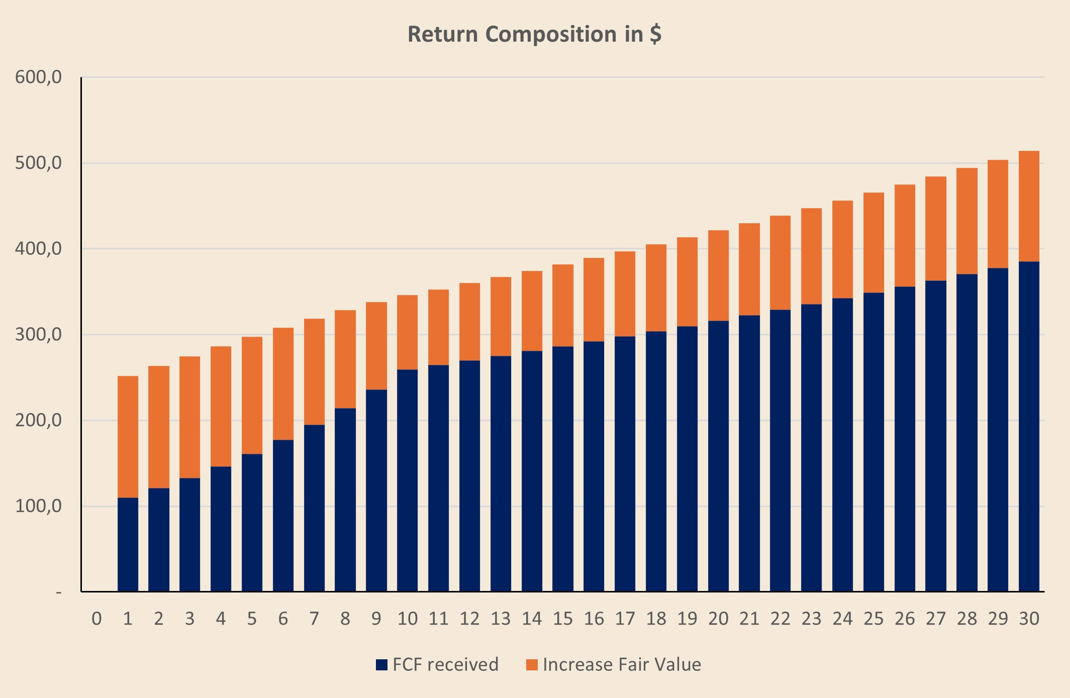
The blue bars show the FCF received during each year (110.0 in year 1). The orange bars show the increase in fair value (142.0 in year 1). Together, they add up to the expected return in dollars (252.0 in year 1), which equals 8% of the beginning fair value in each period.
6. Closing the Loop to the 3 Engines Model
The chart shows the same idea as a percentage of beginning fair value.
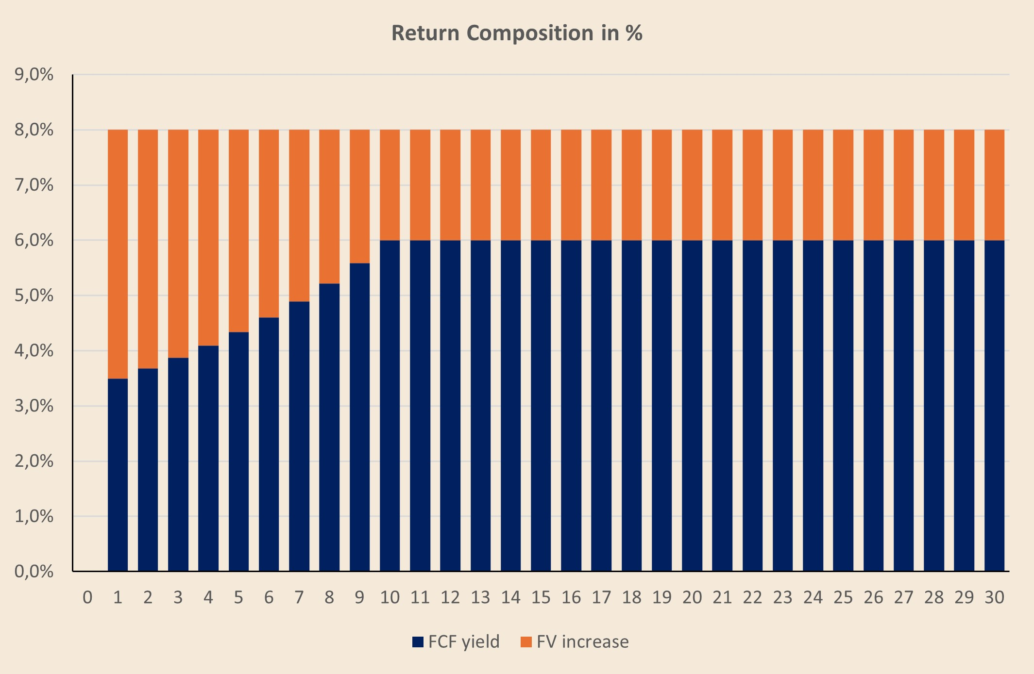
Here, the total bar always adds up to 8% (unsurprisingly). That is the discount rate.
In the early years, a smaller part of the return comes from FCF-yield and a larger part comes from fair-value accretion. The business is still in the high-growth phase, so a meaningful portion of the return comes from the fact that the remaining cash flows move closer and the TV becomes less heavily discounted.
This brings us back to a framework I often use when thinking about shareholder returns: the 3 Engines Model.

Instead of EPS growth, we use FCF-growth. Instead of dividend yield, we use FCF-yield. Instead of the change in the P/E multiple, we use the change in the FCF multiple.
The basic intuition is:
The word “approximately” matters here. Growth and multiple change do not work perfectly additively. A 10% increase in FCF and a 5% decline in the FCF multiple do not simply net to 5%. The higher FCF is applied to a lower multiple, so the two effects interact.
For that reason, the fair-value change is calculated as follows:
In year 1, the company generates 110.0 of FCF on a beginning fair value of 3,150.1. That is a 3.5% FCF yield.
At the same time, FCF growth is 10%.
But the implied FCF multiple falls by 5%.
At year 0, the fair value is 3,150.1 and FCF is 100.0, so the implied multiple is 31.5x.
At year 1, the fair value is 3,292.1 and FCF is 110.0, so the implied multiple falls to 29.9x.
That multiple compression is the model doing exactly what it should do. One year of high growth has been consumed. The business now has nine years of 10% growth left, not ten, i.e. consuming part of the the valuation “premium”.
Once we have reconstructed the fair-value change, we can add the FCF-yield to close the return bridge:
7. Interim Conclusion: What the Fixed 10-Year Case Tells Us
Let’s summarize what the fixed 10-year DCF has shown us.
First, the TV is not a mysterious add-on. It is simply a shortcut for all cash flows after the explicit forecast period. In our base case, the company grows FCF at 10% for ten years and then fades to 2% perpetual growth. Instead of forecasting every cash flow from year 11 into infinity, we calculate one TV at the end of year 10 and discount it back to today.
Second, the year-0 fair value is only a snapshot. In our example, the business is worth 3,150.1 at year 0. But if the business develops as modeled, that value rolls forward over time. The fair value at each point in time is still made up of the same two blocks: the PV of the remaining explicit cash flows plus the PV of the TV.
Third, the return implied by the DCF equals the discount rate if the stock trades at fair value and the cash flows arrive as expected. In our example, that return is 8% per year. But the return is not one single thing. It comes from FCF received during the year plus the increase in fair value.
Fourth, the 3 Engines Model closes the loop. From a FCF perspective, total return can be understood through FCF-yield, FCF growth, and the change in the FCF multiple.
Now we can finally ask the question this article is really about — in case all the DCF mechanics made you forget it for a moment:
What happens if the company is not really a 10-year grower? What if the business can grow at above-average rates for 20 years (or even more) before fading into maturity?
8. The Fixed 20-Year Case: What If the Company Fades Later?
Now we can change one assumption.
In the classic 10-year case, the model assumes that the company grows FCF at 10% for ten years and then fades to 2% perpetual growth. That is the standard DCF structure used by most analysts.
But what if the business is more durable than that?
What if the company can grow FCF at 10% for 20 years or 30 years before fading to 2%?
Importantly, we are not changing the terminal growth rate. We are still using 2% perpetual growth. The business still matures eventually. The only change is the timing of that maturity.
In the 10-year case, the model says:
In the 20-year case, the model says:
Believe it or not, but that one change has a large impact.
The table below turns the exercise into a sensitivity analysis. It shows what fair value looks like across different high-growth periods, from 5 to 30 years. We can recognize our original 10-year case in the highlighted row. Now we compare it with a 20-year high-growth case.
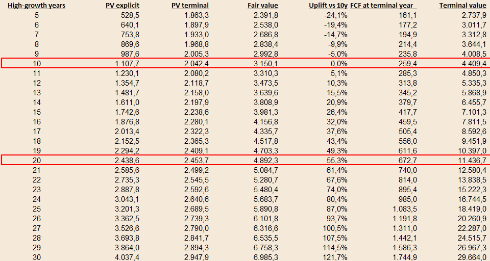
In the 10-year case, the company grows FCF at 10% for ten years and then fades to 2% perpetual growth. The PV of the explicit cash flows is 1,107.7. The PV of the TV is 2,042.4. Together, this gives us a fair value of 3,150.1.
In the 20-year case, the PV of the explicit cash flows increases to 2,438.6, because we now explicitly model another ten years of 10% FCF growth. The PV of the TV also increases to 2,453.7. The TV is much larger in nominal terms, because the company reaches a much higher FCF base before entering the terminal-growth phase. But because this TV is ten years further away, a large part of that nominal increase is offset by additional discounting.
The result is still substantial:
Extending the high-growth period from 10 to 20 years results in a 55.3% increase in fair value.
This is where classic DCF models can undervalue durable compounders.
The model is not mathematically wrong. The TV is not wrong either. The problem is that the model forces the company into maturity too early. In the 10-year case, all growth beyond year 10 is compressed into a 2% terminal-growth assumption. But if the business can still grow at 10% from year 11 to year 20, that extra decade of above-average growth is heavily underrepresented in the classic DCF.
Terminal growth remains at 2% in both cases. The uplift comes from allowing the business to compound at 10% for longer before it enters the terminal-growth phase.
The chart summarizes the practical impact of durability.
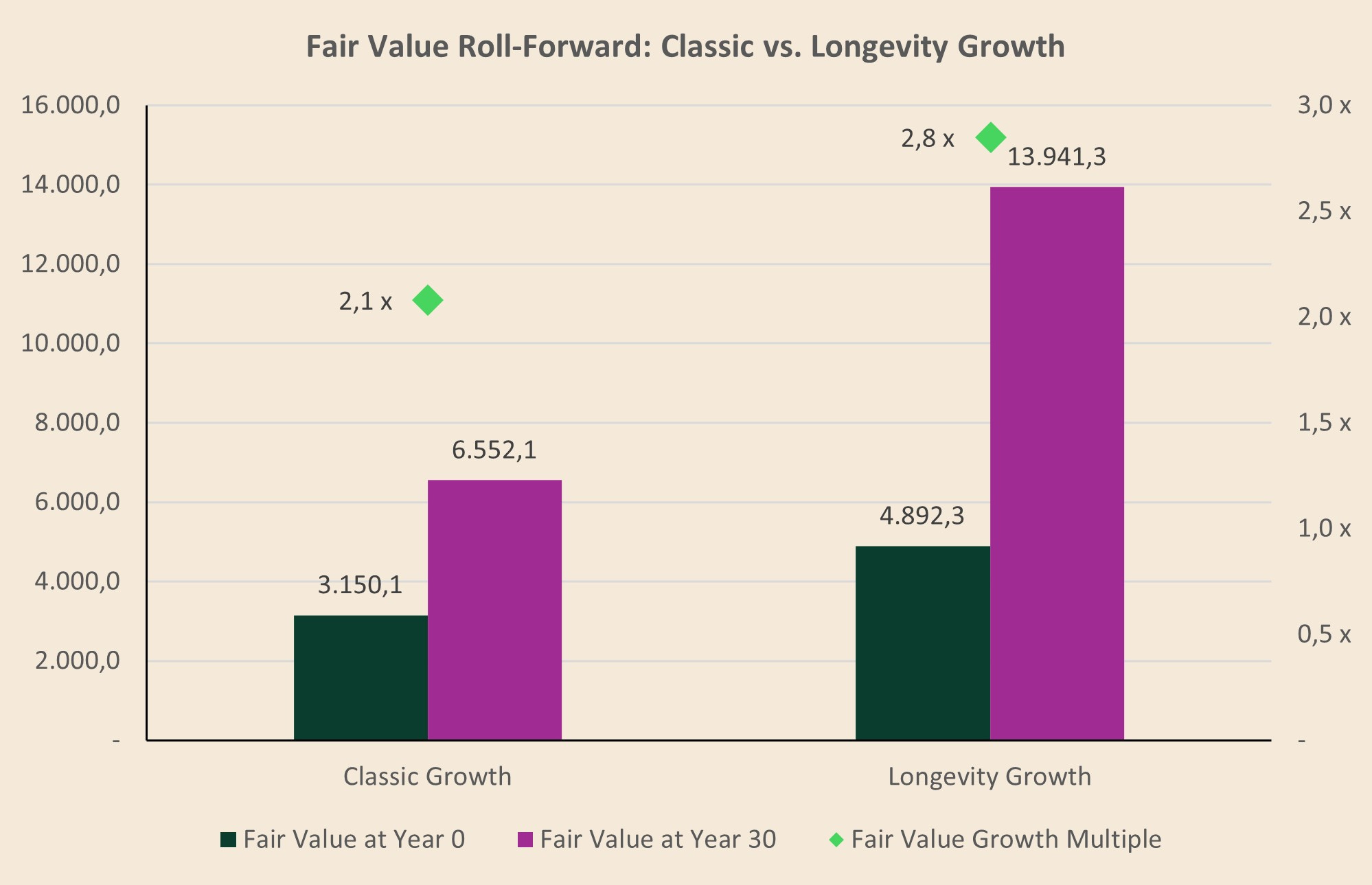
The dark green bars show the fair value today. Extending the high-growth period from 10 to 20 years increases the year-0 fair value from 3,150.1 to 4,892.3.
The purple bars show the fair value at year 30. Here, the gap becomes even larger: 6,552.1 in the classic case versus 13,941.3 in the longevity case.
The green diamonds show the fair value expansion over time. The longevity case does not just start at a higher value; it also compounds to a much higher value because the company spends more years growing at above-average rates before fading into maturity.
The 20-year case also tells us something important about valuation premiums.
In the classic case, fair value increases from 3,150.1 in year 0 to 6,552.1 in year 30. That is a fair-value CAGR of roughly 2.5%.
In the longevity case, fair value increases from 4,892.3 in year 0 to 13,941.3 in year 30. That is a fair-value CAGR of roughly 3.6%.
But this does not mean that the expected shareholder return is only 2.5% or 3.6%. The fair value growth only captures the price appreciation component. The company also generates FCF along the way.
If the stock trades at fair value throughout the period and the cash flows arrive as modeled, the investor’s total return is still the discount rate: 8% per year in both cases.
Importantly, the longevity case does not produce a higher expected return if you pay its full fair value upfront. It produces a higher fair value. The additional durability is capitalized into the starting valuation.
In other words, a longer runway does not magically create excess return once the market fully recognizes it. It creates a higher justified valuation. The excess return opportunity exists only if the market underestimates that runway and prices the business like a 10-year grower when it is actually a 20-year grower.
The longevity case does not automatically mean that investors earn a higher return if they pay the full longevity fair value upfront. If the business is truly worth 4,892.3 and the investor pays 4,892.3, the expected return is still the discount rate. In our example, that is 8% per year.
The difference is that the company is worth more.
A business that can grow FCF at 10% for 20 years is more valuable than a business that can do so for only 10 years. That higher durability is capitalized into the fair value. The 20-year case deserves a higher starting valuation because the company has a longer high-growth runway.
So the higher value is not the same as a higher return.
Fully priced durability gives you a higher justified valuation, but still only the required return. Mispriced durability gives you something more: the required return plus the possibility of a valuation re-rating as the market realizes that the business can compound for much longer than originally assumed.
But the medal has two sides.
The same mechanism can also work in reverse. If the market initially assumes a long high-growth runway and later realizes that growth is fading earlier than expected, the valuation has to adjust downward. In DCF terms, the explicit high-growth period gets shorter. The company is pushed into the terminal-growth phase earlier. The market no longer capitalizes as many years of high growth.
That means the FCF multiple falls. Or, viewed from the other side, the FCF yield rises. A higher FCF yield is just the inverse of a lower valuation multiple. The business may still be a good company. It may still generate strong cash flows. But if the market shortens the assumed growth runway, the valuation premium can compress heavily.
This is exactly what multiple deflation looks like in practice.
Evolution, Copart and Novo Nordisk are good examples. All three were long treated as high-quality, high-growth compounders. But once reported growth slowed, the market began to reassess the duration of that growth. The question shifted from “how fast can this company compound?” to “is the high growth phase over or is the decline in growth temporary?”
In Evolution’s case, revenue growth slowed dramatically from the extraordinary post-2021 levels. At the same time, the forward FCF yield moved sharply higher.

Copart shows a similar dynamic. As growth normalized, the forward FCF yield rose, implying a lower FCF multiple. Again, this does not automatically mean the business quality disappeared. It means the market shortened the implied duration of above-average growth.

Novo Nordisk is a good example of how quickly the market can reassess duration. For years, the stock benefited from the belief that the GLP-1 opportunity could support high growth far into the future. Once investors started to believe that growth might fade earlier than previously assumed, the multiple had to adjust. That is the reverse duration-extension effect: the runway gets shortened, the fade moves closer, and the stock de-rates — whether that reassessment ultimately proves justified or not.

This is why durability is so important.
A great business can look optically cheap after multiple compression, but the key question is whether the market is right to shorten the runway. If the growth slowdown is temporary, the higher FCF yield may represent an opportunity. If the slowdown reflects a structural fade toward maturity, the lower multiple may be justified.
9. The Rolling 10-Year Case: When the Growth Runway Gets Refilled
So far, we have looked at fixed-period DCFs.
In a fixed 10-year DCF, the high-growth period is gradually consumed. At year 0, the company has ten years of 10% growth ahead. One year later, only nine years are left. Five years later, only five years are left. By year 10, the high-growth period is gone and the business has faded into the terminal-growth phase.
That is why the multiple compresses over time. The company may still execute perfectly, but the model is using up the growth runway.
In practice, however, investors rarely think like this.
When an analyst rolls a model forward, they often do not say: “This company now has only nine years of high growth left.” Instead, if the business keeps performing well, they may rebuild the model and again assume another ten years of elevated growth from the new, higher cash-flow base.
That is a very different assumption.
The fixed DCF says: The high-growth period gets consumed.
The rolling DCF says: The high-growth period gets replenished.
This is where durable compounders become interesting.
In our original 10-year case, the year-0 fair value is 3,150.1. If we keep the model fixed, the fair value in year 10 is simply the TV of the original model: 4,409.4. At that point, the high-growth period is over and the company is valued as a mature 2% grower.
But now assume something different.
Assume the company reaches year 10 exactly as expected. FCF has grown from 100.0 to 259.4. But instead of saying “the high-growth period is now over,” the market looks at the business again and concludes: this company still has another ten years of 10% growth ahead.
Then we run a new DCF in year 10.
The starting FCF is now 259.4. From that higher base, we assume another ten years of 10% growth, followed by 2% terminal growth. The recalculated fair value in year 10 is no longer 4,409.4. It is 8,170.6.
The math is simple. The original year-0 fair value was 3,150.1. Ten years later, the recalculated fair value is 8,170.6.
The fair value has therefore compounded at 10% per year. That is not a coincidence. In this rolling 10-year case, the company still receives the same 10-year high-growth FCF multiple (as the maturity profile has not deteriorated), but now on a higher FCF base. The FCF multiple stays constant, while FCF grows by 10%. As a result, fair value also grows by 10%.
That is the power of a “refreshed” runway and why durable compounders can keep surprising investors.
This creates what I would call a duration extension effect. The market does not simply roll the original DCF forward. It extends the period of above-average growth. The growth runway is pushed further into the future, the FCF multiple remains higher for longer, and fair value compounds closer to the growth of the underlying cash flows.
If the company reaches year 10 and still deserves another ten years of high-growth assumptions, it was not a true 10-year grower. It was a longer-duration compounder that the original DCF underestimated.
Fixed 10-year DCF:
FCF grows, but the multiple compresses as the growth runway gets consumed.
Rolling 10-year DCF:
FCF grows, and the multiple can remain elevated because the growth runway gets replenished.
10. Final Thoughts: The Practical Implication
A DCF is useful. But for high-quality compounders, the real work starts where the spreadsheet becomes most fragile: the duration of above-average growth.
The key question is not whether terminal growth should be 2.0% or 2.5%. The key question is how long the business can avoid becoming a terminal-growth business in the first place.
That turns the DCF from a mechanical valuation exercise into a durability exercise (that sounds so intelligent, lol).
The questions become much more specific. How large is the reinvestment runway? How much market share can the company still take? Are incremental returns still high? Is the moat strengthening or weakening? Does the company have pricing power? Is growth capital-light or capital-heavy? Does management have a track record of redeploying cash at attractive returns? Is the business still small relative to the opportunity set?
This is one of the reasons why I appreciate high-quality serial acquirers so much. If the model is decentralized, the acquisition universe is fragmented, the balance sheet is strong, and capital allocation remains disciplined, the runway can be much longer than a standard 10 year-DCF assumes. Can Röko still grow 20 years from now? Very likely. The exact path will be lumpy, but the structural runway is there.
For other companies, the answer is much harder. Can Evolution or Copart still grow at attractive rates 20 years from now? I honestly do not know. The business has been exceptional, but the durability question is more difficult. The runway is less visible. The range of outcomes is wider.
These are the questions that matter.
If the market prices a company like a 10-year grower, but the business keeps proving that it can grow for much longer, the DCF keeps getting extended. The runway gets refilled. The multiple does not compress as quickly. That is where durable compounders can create excess returns.
But the reverse is also true. If the market once assumed a long runway and growth starts fading earlier than expected, the explicit growth period shrinks. The fade into TV moves closer. The multiple compresses. Even a great business can become a poor investment if investors paid for durability that was never really there.
That is why I do not want to use a DCF only as a point estimate.
I want to use it as a framework for asking better questions about longevity.
And that is also exactly how I am approaching my next Deep Dive. The company will remain unnamed for now, but the growth prospects look compelling.
It operates in a highly regulated, mission-critical niche with long product lifecycles, recurring demand, and customer incentives that are not always obvious from the outside. Its market position has been built over decades, not quarters. The business benefits from a large installed base, replacement demand, technical know-how, regulatory approvals, and a value proposition that becomes more relevant when customers are under pressure to reduce costs without compromising reliability.
The upcoming analysis will go deep into the industry structure, regulation, customer incentives, replacement cycles, the long-term durability of the growth runway, and much more. Stay tuned!
Great points and fully agree.
However, as ‘life can only be understood backwards, but must be lived forwards’, question whether it has only theoretical or besides practical application? To put it differently, although a company like GOOGL realised say 20% annualised growth for the past 20 years, reluctant to DCF the same growth for the next 20.